DETECTION OF CEREBRAL EDEMAS AND HEMATOMAS USING EDDY CURRENTS
|
|
|
- Tiit Sikk
- 2 aastad tagasi
- Vaatused:
Väljavõte
1 TALLINN UNIVERSITY OF TECHNOLOGY Faculty of Information Technology Thomas Johann Seebeck Institute of Electronics Chair of Communicative Electronics Madis Ehanurm DETECTION OF CEREBRAL EDEMAS AND HEMATOMAS USING EDDY CURRENTS Master Thesis IEE70LT Supervisor: senior researcher Rauno Gordon Tallinn 2014
2 AUTHOR'S DECLARATION The following master thesis is made by me and me alone. All work of other authors, important positions, and data from different literature used preparing this thesis are cited. This thesis has not been submitted for protecting before.. (date)... (signature) 2
3 DETECTION OF CEREBRAL EDEMAS AND HEMATOMAS USING EDDY CURRENTS Abstract Cerebral edemas and hematomas are an excess accumulation of fluid (blood, in case of hematoma) under the skull in the intracellular or extracellular spaces of the brain. Edemas and hematomas are usually caused by physical traumas or other forms of injury to the brain or head. It is important to detect these pathologies in early stages because as they "grow" they increase ICP and increased ICP can cause (brain)death. Untreated edemas and hematomas can also be held accountable for loss in brains functionality. Usual means in hospitals to discover edemas or hematomas regularly include the use of CT or MRI scanner. The need for a new methodology to detect cerebral edemas or hematomas comes from the fact that many patients cannot be tested using MRI or CT scanners, for example those on life-support. Another means to detect these brain pathologies is to use invasive methods but those methods have many limiting factors. The research team behind the project this thesis is part of, works on creating a methodology and hopefully a prototype to detect the presence of edema or hematoma with non-invasive means. The method proposed to use was detecting the changes in the electric conductivity of the brain by measuring eddy currents induced by a single coil placed above the head. Because it is also important to know what we are simulating and if there exists anything similar this thesis contains overviews of brain and head anatomy and the pathologies we want to detect and also an overview of current non-invasive methods that use electric or magnetic fields for detecting cerebral edemas or hematomas. The main task of this thesis is to validate this methodology via simulations and in case of positive results also optimize the coil for the most effective readout. The main part of the thesis is about simulations: validating software, methodology and optimizing coil parameters. The simulations in this thesis were done with the program Comsol Multiphysics, graphs were done using Microsoft Excel. A comparison between actual measurements of a PCB based planar coil and simulation results showed that the software gives solid and fairly accurate results. Before simulating the head we also needed a head model. To simplify things an axis-symmetric 3
4 model with averaged constant values (as the thicknesses / widths of different tissue layers) were used. Different simulations showed that the changed conductance caused by the presence of edema / hematoma have measurable effect on the coils impedance. Although the differences were in mω given the 1A excitation current we get voltage changes that are measurable. The simulation results were coils impedance values given in the form of a complex number. Although not part of the original task a comparison between different properties (modulus, phase shift, etc.) showed that the biggest percentual difference between edema / hematoma and no pathology were given by the real part of the complex impedance. Simulations to evaluate the effects of different properties to the ability of the coil to detect edema showed that the coil should have wide and low rectangular cross-section and that it should be a bit conic so that the coil will follow the curvature of the head. The number of turns should not be very high but neither very low, and there should be very little free space between the turns. Inner diameter of the coil should be mm. A coil with following properties was proposed: 25 x 3 mm cross section, (-)12 o angle, 100 turns, wire AWG22 and an inner diameter of 20 mm. The thesis proved the theoretical possibility of using coils to detect different brain pathologies and gave us an optimal coil for the task. Future tasks ahead include testing the method against the variability of the human head parameters (skull thickness, blood vessels, etc), providing a better method to assess the difference caused by the presence of edema / hematoma and creating an actual device. When the device is ready the coil will need reassessing. More precisely the effects of the coils SRF caused by parasitic capacitance need further research to make sure that the highest difference values showed by simulations would actually be measurable. 4
5 AJUÖDEEMI PÖÖRISVOOLUSID JA HEMATOOMI TUVASTAMINE KASUTADES Annotatsioon Ajuödeemid ja hematoomid on liigse vedeliku kogunemine (hematoomi puhul vere) kolju all rakusiseses või rakuvälises ruumis ajus. Ödeemide ja hematoomide peamisteks põhjustajateks on füüsiline trauma või muud aju või pea vigastused. Nende avastamine varases järgus on oluline kuna nende kasvades hakkavad nad suurendama intrakraniaalset rõhku ja suurenenud ajusisene rõhk võib põhjustada (aju)surma. Ravimata ödeemid ja hematoomid võivad põhjustada aju funktsionaalsuse kahanemist. Tavalised vahendid haiglates ödeemi ja hematoomi avastamiseks on kompuutertomograafia või magnetresonantstomograafia. Vajadus uue metoodika järele ajuödeemide / hematoomide tuvastamiseks tuleb asjaolust et tomograafia kasutamine on paljude patsientide puhul välistatud, nt patisendid kes on ühendatud elul-hoiu seadmetega. Teine viis tuvastada neid aju patoloogiad hõlmab invasiivseid meetodeid, kuid neil on palju piiravaid faktoreid. Uurimismeeskond, kes on projekti taga millest ka see lõputöö on üks osa, püüab luua metoodikat ja loodetavasti ka protüüpi mitteinvasiivseks ajuödeemi ja hematoomi tuvastamiseks. Ettepanek metoodika osas oli mõõta patoloogia poolt põhjustatud aju koe juhtivuse muutusi, mõõtes pea peale asetatud mähise poolt indutseeritud pöörisvoolusid. Kuna on oluline teada, mida simuleerida ja kas juba eksisteerib midagi sarnast, siis sisaldab käesolev lõputöö nii ülevaadet aju ja pea anatoomiast ja patoloogiatest kui ka praegustest mitteinvasiivsetest ödeemi ja hematoomi mõõtemeetoditest mis kasutavad elektri- või magnetvälju. Käesoleva töö peamine ülesanne oli siiski valideerida väljapakutud metoodika erinevate simulatsioonide kaudu ning positiivsete tulemuste korral ka optimeerida mähist võimalikult hea mõõtetulemuse saamiseks. Põhiosa tehtud tööst moodustavad erinevad simulatsioonid : tarkvara ja metoodika valideerimine ning mähise optimeerimine. Simulatsioonid sooritati programmiga Comsol Multiphysics, graafikud on loodud Microsoft Exceli abil. 5
6 Võrdlus tasapinnaline trükkplaadimähise reaalsete mõõtetulemuste ja simulatsioonitulemuste vahel näitas, et tarkvara annab arvestatavaid ja üsna täpseid tulemusi. Enne patoloogiate tuvastamise simuleerimist oli vaja ka pea mudelit. Lihtsustamise huvides kasutati telgsümmeetrilist keskmistatud kihtide paksustega pea mudelit. Erinevad simulatsioonid näitasid, et hematoomi / ödeemi poolt põhjustatud muutunud juhtivus omab mõõdetavat efekti mähise impedantsile. Kuigi erinevused olid suurusjärgus mω, siis antud ühe ampri suuruse ergutusvoolu juures saame pinge muutuseid, mis on mõõdetavad. Simulatsiooni tulemuseks saime pooli impedantsi kompleksarvu kujul. Kuigi see ei olnud osa algsest ülesandest, siis võrdlus erinevate omaduste vahel ( moodul, faasinihe jne ) näitas, et kõige suurema tuvastava protsentuaalse erinevuse patoloogilise ja normaalolukorra vahel saame kui võrrelda kompleksimpedantsi reaalosa. Simulatsioonid, mille ülesandeks oli hinnata mähise erinevate omaduste mõju mõõtetulemuste erinevusele, näitasid, et mähise ristlõige peaks olema lai ja madal ristkülik. Mähis peaks olema keritud selliselt et ta järgiks pea kumerust. Keerdude arv ei tohiks olla väga suur, kuid ka mitte väga väike, lisaks peaks keerdude vahel minimaalselt tühja ruumi. Sisediameeter peaks olema vahemikus mm. Välja sai pakutud näidismähis järgmiste omadustega: 25 x 3 mm ristlõige (-)12 o nurgaga, 100 keerdu traati AWG22, sisemine läbimõõt 20 mm. Käesolev magistritöö tõestas teoreetilise võimaluse kasutada mähist leidmaks eri aju patoloogiad ning andis optimaalse mähise selle ülesande täitmiseks. Tulevikus tuleb edasi testida meetodi töökindlust muutuvate inimpea parameetrite korral (nt kolju paksus, veresooned jne), tuleb leida parem meetod hindamaks patoloogilist olukorda / mõõtetulemuste erinevust, lisaks tuleks välja töötada ka reaalne prototüüp. Kui seade on valmis, tuleks mähist uuesti hinnata. Täpsemalt tuleks uurida parasiitmahtuvuse poolt põhjustatud omavõnkesagedust ning teha kindlaks, kas simuleeritud suurimad mõõtetulemuste erinevused on ka reaalsete mõõtmiste korral korratavad. 6
7 GLOSSARY OF TERMS AND ABBREVIATIONS Eddy currents electric currents induced by changing magnetic field in the conductor (in our case the conductor is a coil and the changing magnetic field is caused by coil's alternated excitation current). Pathology the conditions and processes of a disease or any deviation from a healthy, normal, or efficient condition, also the science or the study of the origin, nature, and course of diseases Traumatic brain injury (TBI) also known as intracranial injury, in this thesis term brain trauma may also be used, TBI is usually caused by external forces. In this thesis this term is used for cerebral edemas and brain hematomas. Cerebrospinal fluid (CSF) a water-like fluid found in the brain and spine, acts as a cushion for the brain's cortex, providing a basic mechanical and immunological protection to the brain inside the skull. Cerebral edema excess accumulation of fluid (mostly a mixture of blood and CSF) in the brain; also written as oedema. Epidural hematoma buildup of blood between dura mater and skull. Subdural hematoma buildup of blood between dura mater (adheres to the skull) and arachnoid mater (envelops the brain). Intracranial pressure (ICP) pressure inside the skull and thus in the brain tissue and cerebrospinal fluid (CSF), normally 7 15 mmhg for a supine adult; elevated ICP is one of the most damaging aspects of brain trauma and is directly correlated with poor outcome. Magnetic resonance imaging (MRI) medical imaging technique used in radiology to investigate the anatomy and function of the body, uses strong magnetic fields to detect the movement of excited hydrogen atoms. Electrical Impedance Tomography (EIT) medical imaging technique where image of the conductivity/permittivity of part of the body is inferred from surface electrical measurements. 7
8 Computed Tomography (CT) any computer-aided tomographic process, in this context and medically usually x-ray computed tomography. It uses irradiation to produce three-dimensional representations of the scanned object both externally and internally. Eddy current testing (ECT) methodology, that uses electromagnetic induction to detect flaws in conductive materials. Eddy-current testing can detect very small cracks in or near the surface of the material. It is also useful for making electrical conductivity and coating thickness measurements. Self-resonance frequency (SRF) in case of inductors the frequency where parasitic capacitance of the inductor resonates with the inductance and the inductor becomes a parallel resonant tuned circuit. (actual inductor could be viewed as a LC parallel circuit). Non-destructive testing (NDT) a wide group of analysis techniques used in science and industry to evaluate the properties of a material, component or system without causing damage CG coil group; one way to simulate multi-turn coil using Comsol Multiphysics is to create number of single-turn coils and to use them as a coil group MTC multi-turn coil, another and simpler way to simulate multi-turn coil using Comsol Multiphysics. MOD short for modulus (absolute value of complex signal, in our case impedance) used when comparing simulation results. RE short for real part of the complex signal (in our case impedance); used when comparing simulation results. IM short for imaginary part of the complex signal (in our case impedance); used when comparing simulation results. 8
9 LIST OF SCHEMES AND FIGURES Figure 1.1 Cranial bones Figure 1.2 Protective coverings of the brain [11] Figure 1.3 Gray and white mater distribution in the brain [11] Figure 1.4 Cytotoxic edema [5] Figure 1.5 Development of an epidural hematoma [6] Figure 1.6 Development of a subdural hematoma [6] Figure 1.7 Epidural hematoma (left) vs. subdural hematoma (right) [9] Figure 2.1 Theoretical relative phase shift in brain tissue [18] Figure 2.2 VEPS clinical Head/coil; a patient wearing it [19] Figure 2.3 Scalar classifier plot based on subjects β and γ value [19] Figure 2.4 Initial conditions of current and magnetic fields [30] Figure 2.5 Parasitic capacitances in a coil Figure 3.1 Comsol Multiphysics program-tree Figure 3.2 Measured results vs. simulated results (Coil group) Figure 3.3 Coils cross-section for simulation model Figure 3.4 Signal properties over frequency range Figure 3.5 Percentual differences between signal components Figure 3.6 Difference in real part of impedance in Ohm's (edema no edema) Figure 3.7 3D simulation result for 2D axissymmetric model Figure 3.8 Simulation model for validating method Figure 3.9 Modulus of the impedance Figure 3.10 Difference of moduluses (edema vs. no edema) Figure 3.11 Phase shift (φ) and difference in phase shift in the presence of edema Figure 3.12 Real parts of simulated complex impedance Figure 3.13 Difference of real parts of impedance (edema no edema) Figure 3.14 Imaginary parts of simulated complex impedance Figure 3.15 Difference of imaginary parts of impedance (edema no edema) Figure 3.16 Percentual changes in impedance properties caused by edema Figure 3.17 Percentual differences for various coil shapes Figure 3.18 Different coil shapes simulated Figure 3.19 Coils cross-section measurements effect on the difference between edema and normal situation Figure 3.20 Differences for constant surface area
10 Figure 3.21 Differences for constant aspect ratio Figure 3.22 Differences for constant height Figure 3.23 Differences for constant width Figure 3.24 Inner diameters effect on the difference between edema and normal state. 58 Figure x 8.66 mm coil differences for variable inner diameter Figure x 3 mm coil differences for variable inner diameter Figure 3.27 Differences for inner diameters of 10; 20; 30 mm Figure 3.28 Coils number of turns effect on the coils sensitivity to edema (coil 1) Figure 3.29 Coils number of turns effect on the coils sensitivity to edema (coil 2) Figure 3.30 Coils number of turns effect on the coils sensitivity to edema with constant coil density Figure 3.31 Axis-symmetric models for edema and hematoma Figure 3.32 Simulated differences for example coil Figure 3.33 Comparison of previously suggested 8.66 x 8.66 mm, d inner =30 mm, 100 turn coil Figure A.1 Wet skin conductivity and permeability (measured vs. calculated) Figure A.2 Fat conductivity and permeability (measured vs. calculated) Figure A.3 Cortical bone conductivity and permeability (measured vs. calculated) Figure A.4 Dura conductivity and permeability (measured vs. calculated) Figure A.5 Grey matter conductivity and permeability (measured vs. calculated) Figure A.6 White matter conductivity and permeability (measured vs. calculated) Figure A.7 CSF conductivity and permeability (measured vs. calculated) Figure A.8 Blood conductivity and permeability (measured vs. calculated) Figure A.9 Classical model of real-life inductor LIST OF TABLES Table 3.1 Frequency values for conductance/permittivity calculations Table 3.2 Properties of the measured/simulated coil Table 3.3 Important properties of layers used in simulation model Table 3.4 Simulation results for coils impedance (Z) Table 3.5 Common properties for coils Table 3.6 Parameters for coil cross-sections measurement simulations Table 3.7 Parameters for coils inner diameter simulation Table 3.8 Coil parameters for optimizing the number of turns Table A.1 Parameters for finding tissues electrical properties Table A.2 Nagaoka's coefficients [34]
11 CONTENTS AUTHOR'S DECLARATION... 2 DETECTION OF CEREBRAL EDEMAS AND HEMATOMAS USING EDDY CURRENTS... 3 AJUÖDEEMI JA HEMATOOMI TUVASTAMINE KASUTADES PÖÖRISVOOLUSID... 5 LIST OF SCHEMES AND FIGURES... 9 LIST OF TABLES CONTENTS INTRODUCTION BIOLOGICAL BASIS Human head anatomy Overview of brain injuries Cerebral edema Epidural hematoma Subdural hematoma TECHNICAL BASIS Overview of non-invasive methods for detecting brain traumas EIT (Electronic Impedance Tomography) MREIT (Magnetic Resonance EIT) MIT (Magnetic Induction Tomography) Volumetric Electromagnetic Phase-Shift Spectroscopy REG (Rheoencephalography) MAT-MI (Magneto-Acoustic Tomography with Magnetic Induction) Theoretical basis of measurement using eddy currents Self-resonance frequency of a coil (SRF)
12 3. SIMULATIONS Overview of COMSOL Multiphysics [27] Frequency dependent electrical properties of tissues Validation of simulations Simulation methods in Comsol Comparison of multi-turn coil simulation methods Choosing the Right Space Dimension Method validation Coil optimization Coil shape configuration Measurements of the cross-section of the coil Inner diameter for the coil Number of turns Optimized coil Testing optimized coil CONCLUSIONS DISCUSSION REFERENCES / SOURCES A. APPENDIXES Appendix 1: Calculation of tissues electrical proeprties [29] Appendix 2: Calculating solenoids SRF
13 INTRODUCTION The following master thesis is a part of a bigger project between PERH (North Estonia regional hospital) ELIKO Technology Competence Centre in Electronics-, Information and Communication Technologies and TUT (Tallinn University of Technology). This project unites scientists, researchers, doctors and students from aforementioned facilities. The objective of this taskforce is to find a new solution to effectively and noninvasively detect cerebral edemas and hematomas or changes in ICP (intracranial pressure) and to do this cheaply and simply. This thesis is also closely related to Rauno Gordon's Estonian Science Foundation grant project g9394 "Advancing the electric tissue diagnostic methods by understanding the influence of vascular system dynamics" ("Elektriliste kudede diagnostikameetodite arendamine veresoonkonna dünaamilisi mõjutusi arvestades", in estonian). This thesis focuses mainly on the idea of detecting cerebral edemas or brain hematomas using coils on patients head. Because of a difference in electrical properties of different human tissues the eddy currents induced in human head are different when the pathology is present compared to when it is not. Thanks to previously mentioned fact we hope to detect edema/hematoma when measuring the coil's voltage or impedance, given that the coil's excitation current remains constant. The main task of this thesis is to validate this method and to find the best properties for a measuring coil, to gain measureable signals. 13
")
14 1. BIOLOGICAL BASIS The following chapter will guide us through the anatomy of a human head and specifically brain. To be able to detect different types of brain injuries being familiar with the anatomy and anatomical processes of human head and brain both in normal states as well as in pathological (injured) states are necessary Human head anatomy This chapter is about the build of a human head. It gives a basic overview of conditions before simulating can start. Different layers and different widths can easily change the outcome of future measurement because of differences in biological and electrical properties. The skeletal framework of head and neck is made up of skull, hyoid bone and cervical vertebrae. The term skull includes the mandible (lower jawbone) and the cranium. Cranium is often used to describe the part of the skull containing the brain. In this thesis we are therefore only interested in the cranium. Cranium is actually comprised by eight bones (parietal and temporal which are paired; frontal, sphenoid, ethmoid, occipital - unpaired). [10] Figure 1.1 Cranial bones 14

15 There are also additional protective layers inside the skull. The cranial meninges surround the brain. They are continuous with the spinal meninges, have the same basic structure, and bear the same name: the outer dura mater, the middle arachnoid, and the inner pia mater. Blood vessels, that enter brain tissue pass along the surface of the brain, and as they penetrate inward, they are surrounded by a loose-fitting layer of pia mater. Three extensions of the dura mater separate parts of the brain: the falx cerebri separates the two hemispheres of the cerebellum; and the tentorium cerebelli separates the cerebrum from the cerebellum. [11] Figure 1.2 Protective coverings of the brain [11] In figure above we have anterior view of frontal section through skull showing the cranial meninges which protect the brain inside the skull. As is widely known, brain consists of many parts, cerebrum, brainstem, cerebellum and they are often divided into many different sub-parts based on what task(s) they are responsible for etc. Concerning this thesis lobes and/or functional areas are not of interest rather the interest lies with different tissue types and their distribution inside the skull. 15

16 Brain consists basically of two types of tissue, white and gray matter. The white matter is aggregations of myelinated and unmyelinated axons of many neurons. The whitish color of myelin gives white matter its name. The gray matter of the nervous system contains neuronal cell bodies, dendrites, unmyelinated axons, axon terminals, and neuroglia. It appears grayish, rather than white, because the Nissl bodies impart a gray color and there is little or no myelin in these areas. Blood vessels are present in both white and gray matter. In the brain, a thin shell of gray matter covers the surface of the largest portions of the brain, the cerebrum and cerebellum. [11] Figure 1.3 Gray and white mater distribution in the brain [11] 16

17 1.2. Overview of brain injuries This chapter focuses on giving an overall overview of cerebral edemas and brain hematomas (both epidural and subdural hematomas) which are the main / only types of brain injuries we are interested in detecting with the simulations conducted as part of this thesis Cerebral edema Cerebral edema is an excess accumulation of fluid in the intracellular or extracellular spaces of the brain. [1] Cerebral edemas can occur when: blood brain barrier or the blood cerebrospinal fluid (CSF) barrier break down (allowing fluid to accumulate in the brain's extracellular space), metabolism is altered which may cause brain cells to retain water, dilution of the blood plasma which may cause excess water to move into brain cells. Cerebral edemas are usually caused by physical traumas or other forms of injury to the brain. [2] Cerebral edemas are traditionally broadly divided into vasogenic cerebral edema (an extracellular edema, blood-brain barrier disrupted, mainly affects the white matter through leakage of fluid out of capillaries, mostly seen around brain tumors) and cytotoxic cerebral edema (an intracellular edema, blood-brain barrier is intact, mainly affects grey matter, happens due to a cellular swelling from lack of ATP). [4] Figure 1.4 Cytotoxic edema [5] The reason, why it is important to detect cerebral edemas is that it is a significant cause of morbidity and mortality in diverse disease states as it often causes rise in ICP. 17

18 Epidural hematoma Epidural hematoma happens when patient bleeds into the epidural space due to detachment of the outer dural sheath from the skull and rupture of a meningeal artery Epidural hematomas can sometimes also be of venous origin.[8] Epidural hematoma usually results from a blow to the head with skull fracture and, unless treated promptly, can be fatal. Occurs in 1% to 2% of head injuries. The middle meningeal arteries reside in grooves in the inner table of the bone between the dura and the calvaria, and their branches splay across the temporal parietal area. The temporal bone is one of the thinnest bones of the skull and is particularly vulnerable to fracture, so seemingly minor trauma may fracture the bone, which may in turn lacerate branches of the middle meningeal artery, resulting in a life-threatening epidural hemorrhage. [6] Transection of the middle meningeal artery permits the escape of blood under arterial pressure into the epidural space, thereby separating the dura from the calvaria. The dura is tightly bound to the calvarium at the coronal suture lines; therefore, the epidural blood accumulation will not extend beyond the suture lines. This leads to a lens-shaped accumulation of fresh blood that stops at the coronal suture lines. Epidural hematomas are invariably progressive. Intracranial pressure increases fast, leading to herniation. When not recognized and evacuated, may be fatal in 24 to 48 hours. [6,7] Figure 1.5 Development of an epidural hematoma [6] 18

19 In the figure above we can see a laceration of a branch of the middle meningeal artery by the sharp bony edges of a skull fracture initiates bleeding under arterial pressure that dissects the dura from the calvaria and produces an expanding hematoma. If the hematoma is not evacuated, lethal Duret' hemorrhages will occur Subdural hematoma Subdural hematomas appear when patient bleeds into the subdural space. They are often accompanied by focal contusion of the underlying brain. Frequently located in the temporal region. [8] Subdural hematomas are typically of venous origin, resulting from stretching or tearing of cortical veins that traverse the subdural space en route to the dural sinuses. They may also result from disruption of penetrating branches of superficial cerebral arteries. Because the inner dural layer and arachnoid are not as firmly attached as the structures that make up epidural space, the subdural hematoma typically extends over a much larger area compared to epidural hematoma. [9] Subdural hematoma is a significant cause of death after head injuries from falls, assaults, vehicular accidents and sporting mishaps. The subdural hematomas expand slower than epidural hematomas, still never mind that the clinical tempo is slower, once critically increased ICP is attained, clinical deterioration and death can occur rapidly. [6] Figure 1.6 Development of a subdural hematoma [6] 19

20 In the part A of the previous figure we can see that when a head trauma happens, the dura moves with the skull and the arachnoid moves with the cerebrum. As a result, the bridging veins are sheared as they cross between the dura and the arachnoid. Venous bleeding creates a hematoma in the expansive subdural space. Subsequent transtentorial herniation is life threatening. In part B we can see the right hemisphere exhibiting a large collection of blood in the subdural space, owing to rupture of the bridging veins. Figure 1.7 Epidural hematoma (left) vs. subdural hematoma (right) [9] Figure above shows an Axial CT scan from a patients head with both epidural hematoma (left side) and subdural hematoma (right). It demonstrates the differences in shape between both hematoma types. Also notice the soft tissue swelling outside the scalp on the left side next to the epidural hematoma.[9] 20
21 2. TECHNICAL BASIS 2.1. Overview of non-invasive methods for detecting brain traumas Since this thesis is mostly about researching and validating the possibility to detect (previously mentioned) brain injuries using eddy currents, this chapter only focuses on methods and devices which use electric or magnetic fields/forces. Furthermore, this chapter only focuses on methods that detect or will be able to detect (as some are still sort of experimental) cerebral edemas or hematomas non-invasively. Invasive methods are discarded since they do not belong in our main area of interest. Also, currently, the means to detect progressive cerebral edema in vivo include the use of intracranial pressure (ICP) monitors and serial radiological studies. However, ICP measurements exhibit a high degree of variability, and ICP monitors detect edema only after it becomes sufficient to significantly raise ICP. [3] Which is why in this chapter methods which rely on ICP measurement are discarded EIT (Electronic Impedance Tomography) Electrical Impedance Tomography (EIT) is a medical imaging technique in which an image of the conductivity or permittivity of part of the body is inferred from surface electrical measurements. Typically, conducting electrodes are attached to the skin of the subject and small alternating currents are applied to some or all of the electrodes. The resulting electrical potentials are measured, and the process may be repeated for numerous different configurations of applied current. EIT has the potential to be relevant in medical diagnostics. It could be used for detecting breast cancer [13] or monitoring brain function [14]. and possibly stroke. However, it is not yet routinely used because it lacks spatial resolution comparable to MRI or CT. Its key advantage is its temporal resolution, which is in the order of milliseconds. [15] 21
22 As a means of validating the use of EIT on the human brain, the UCL group performed a number of measurements from human volunteers who were subject to visual, motor, and somatosensory stimuli to assess the applicability of EIT to the problem of imaging functional activity in the human brain [12]. Impedance/conductance changes in the brain are usually dependent on the blood voulme however, higher conductivity measurement could also refer to brain hematomas or cerebral edema MREIT (Magnetic Resonance EIT) Magnetic resonance electrical impedance tomography is a recently developed medical imaging modality visualizing conductivity images of an electrically conducting object. MREIT was motivated by the image reconstruction problems of EIT. Numerous experiences have shown that practically measurable data sets in an EIT system are insufficient for a robust reconstruction of a high-resolution static conductivity image. [16] MREIT system was proposed in the early 1990s to use the internal data of magnetic flux density B = (B x, B y, B z ), which is induced by an externally injected current. MREIT uses an MRI scanner as a tool to measure the B z component of the magnetic flux density, where z is the axial magnetization direction of the MRI scanner. In 2001, a constructive B z -based MREIT algorithm was developed and its numerical simulations showed that high-resolution conductivity image reconstructions are possible. Since then, imaging techniques in MREIT have advanced rapidly and have now reached the stage of in vivo animal and human experiments. [16] MREIT basically combines MRI and EIT. In MREIT, a reconstruction of the crosssectional current density and conductivity (or resistivity) images of human body with high spatial and contrast resolution can be obtained. Using low-frequency magnetic resonance current density imaging (shortly LF-MRCDI) technique where we acquire MR images with external current injection through surface electrodes, we first obtain images of internal magnetic flux density distribution. This internal information transforms the ill-posed inverse problem of an EIT into a well-posed one in MREIT. As this is a relatively new image method, there are still a number of technical difficulties to 22
23 overcome. The main constraint is the amount of injected current required, which at present is on the order of 15 ma [17] MIT (Magnetic Induction Tomography) MIT is another variation of EIT. It detects very small changes using planar gradiometers, low-noise amplifiers and digital signal processing to achieve high signal to noise ratio. The MIT-systems usually do not use the excitation coil for measurement at the same time. They pick up generated magnetic field by other coils. Generally the changes in the generated magnetic field are orders of magnitudes smaller than the original generated field, therefore the potential generated in the secondary coil is several orders of magnitude smaller than the original signal itself. Some special arrangements have been experimented with, that are aimed for overcoming this sensitivity problem. An example of special coils are gradiometers or planar gradiometers [21]. They help to reduce the primary coils interference into the secondary or receiving coils. Gradiometers are basically 2 coils side-by-side like figure-8 running in opposite directions and connected in the middle forming one long coil that runs many turns one way, then many turns the other way [21],[22]. This approach helps to bring the sensitivity up and frequencies down for more precise signal analysis. Although the MIT would seem like a nice non-invasive and contactless medical visualization modality, it is still in very early stages and the imaging capability has not been validates yet on healthy individuals or patients. 23
24 Volumetric Electromagnetic Phase-Shift Spectroscopy This method is described in more details compared to other brain trauma detecting methods in chapter 2.1. because it resembles the idea and direction the project this thesis is part of is heading the most (compared to other methods described here). Therefore some data in this chapter could be used as reference points for our simulations. Cesar A Gonzales, Boris Rubinsky et.al. [18],[19] have developed a magnetic spectroscopy system to measure total brain impedance with eddy currents with frequencies from 1MHz up to 1GHz. Below are the results from theoretical study and physical phantom measurement set-up. Figure 2.1 Theoretical relative phase shift in brain tissue [18] Figure above shows theoretical phase shift in brain tissue as a function of frequency for various ratios of volumes of normal brain tissue to brain tissue with edema. The frequency is in a logarithmic scale. It shows the difference between the calculated phase 24
![shift in brain tissue with various degrees of edema and the calculated phase shift in the case with 100% brain tissue, as a function of frequency. [18] Figure 2.](/docs-images/115/214004561/images/25-0.jpg "2 VEPS clinical Head/coil; a patient wearing it [19] The VEPS (Volumetric Electromagnetic Phase-Shift Spectroscopy) system that Gonzales's team has prepared consists of a smaller excitation coil on")
25 shift in brain tissue with various degrees of edema and the calculated phase shift in the case with 100% brain tissue, as a function of frequency. [18] Figure 2.2 VEPS clinical Head/coil; a patient wearing it [19] The VEPS (Volumetric Electromagnetic Phase-Shift Spectroscopy) system that Gonzales's team has prepared consists of a smaller excitation coil on the top of the patient s head and a larger receiving coil around the patient s head. R1 = 3.2 cm and R2 = 11 cm, separated by a distance of 10 cm. Both coils were built from ten turns of magnet wire AWG22 (Ø = mm, S Ø =0.326 mm 2, resistance = Ω/km) rolled on a plastic harness designed for an adult human head (figure above). To avoid inductive pickup the leads of the coils are twisted. Scientists behind the VEPS have measured 46 healthy volunteers and 8 patients with brain edema or hematoma and have found a way to separate the groups with using their own special β-integration and γ-integration values. [19] Next figure is a scalar classifier plot of each experimental subject in terms of two values for that subject, β and γ. Each data point represents a subject. Healthy volunteers, patients with brain condition of edema and of hematoma are marked with different symbols. It shows that VEPS is able to detect not only if the patient has a brain trauma but also the type of the trauma. [19] 25
26 Figure 2.3 Scalar classifier plot based on subjects β and γ value [19] REG (Rheoencephalography) Rheoencephalography is a method to assess blood flow in the brain by electric measurements with electrodes applied to the scalp. It is basically an electric impedance measurement on the head. The measured signal actually reflects blood content change or blood volume change in the head locations under the electrodes and the flow parameters have to be determined from that. The physical basis of the REG measurement is based on the fact that blood and cerebrospinal fluid are better conductors than the brain or other 'dry' tissue. The REG signal reflects the impedance change: during blood inflow into the cranial cavity, electrical conductivity increases as represented by increasing REG pulse amplitude. The REG pulse wave represents only a small percentage of the total electrical impedance. An identical change in electrical impedance occurs in a pulse wave generated during impedance measurements on peripheral sites (e.g. leg, arm). [23] Typically, Doppler ultrasound is used in clinical practice to measure CBF and cerebral hemodynamic reserve. The fact that a REG device would be much more cost efficient 26
27 than Doppler ultrasound or a brain mapping device such as the PET scan, explains why REG monitoring has potential for use in diagnosing cerebrovascular alterations measuring cerebral hemodynamic reserve. [23] REG is not a widely used method, but it's been in development for a long time period. Main help for our project is that it is safe to assume that researchers have found many useful ways to analyze brain parameters noninvasively with electric measurements MAT-MI (Magneto-Acoustic Tomography with Magnetic Induction) MAT-MI is a method developed recently in the last decade to reconstruct anatomical images of patients using a magnetic field, eddy currents and acoustic measurements. In MAT-MI, the object to be imaged is placed in a static magnetic field, while pulsed magnetic stimulation is applied in order to induce eddy current in the object. In the static magnetic field, the Lorentz force acts upon the eddy current and causes acoustic vibrations in the object. The propagated acoustic wave is then measured around the object to reconstruct the electrical impedance distribution. [24] Scientists have analyzed MAT-MI and found that when imaging nerve or muscle, electrical anisotropy can have a significant effect on the acoustic signal and must be accounted for in order to obtain accurate images. [25] 27
28 2.2. Theoretical basis of measurement using eddy currents Not to be misguided, the method under discussion is actually not about measuring eddy currents, rather the changes in coil's impedance caused by eddy currents, given that coil's excitation current remains constant. This chapter is about the basics of using coils for measuring conductivity, since changes in conductivity are our main hope for discovering cerebral edemas and brain hematomas. The method proposed to detect brain traumas is very similar to a method used in industries for sorting materials, measuring and controlling dimensions of tubes, sheets, rods, coating thickness etc. This method is called eddy current testing (ECT). [30] In ECT an alternating current is made to flow in measuring coil. Alternating current in turn produces an alternating magnetic field around the coil. As this coil is brought close to electrically conductive material (usually metal, in our case biological tissues) it induces an eddy current flow in the material due to electromagnetic induction (figure below). Figure 2.4 Initial conditions of current and magnetic fields [30] These currents are generally parallel to coils winding. The presence of any defect (when measuring metals) disturbs the eddy current flow (in our case the presence of edema/hematoma actually increases eddy currents). However because the eddy currents 28
29 are produced by an alternating magnetic field they are also alternating and therefore create an alternating magnetic field (which has opposite direction to original magnetic field) around the area where eddy currents are flowing. Those secondary magnetic fields can be detected as a voltage across a second coil or by a change of impedance of the first coil. [30] The impedance change in ECT is mainly affected by changes in electrical conductivity, magnetic permeability and geometry of the material, test frequency and the spacing between the coil and the measured object. The test results are also affected by coils parameters (width, height, radius, number of turns, etc). [30] In our case the biggest contributors to the change in coils impedance (when comparing results between the cases when edema/hematoma is present vs. when it is not) are conductance and permittivity values of different tissues. Permeability is of no importance because it has constant value for all human tissues. Also coils parameters and measuring frequency/frequencies play an important role when trying to get as big difference as possible comparing pathological stage to normal. Tissue parameters are known values. The values for coil parameters will hopefully emerge from simulation results. 29
 insulator in the free room between wires, this resembles the build of a capacitor (dielectric between two conducting plates)")
30 2.3. Self-resonance frequency of a coil (SRF) Before starting simulating it is important to mention coils SRF. As it is known coils have parasitic capacitance. Coils cross-section is basically a grid of conductors with air and (wire) insulator in the free room between wires, this resembles the build of a capacitor (dielectric between two conducting plates) and therefore acts as a (parasitic) capacitor. Figure 2.5 Parasitic capacitances in a coil Figure above shows a cross-section of a 20x8 turn coil. Left bottom corner shows parasitic capacitances for one turn of the coil. The parasitic capacitance might not be that big but it is a problem, as it means that at some frequency any coil will start (self)resonating and therefore above that frequency it is difficult if not next to impossible to assess what to expect from measuring results. Also the simulation software does not take parasitic capacitance into consideration therefore simulation results will not be accurate around and above the SRF. Based on different literature it is possible to assess the SRF of a solenoid using different formulas, however when we have a coil with different build we can expect the SRF to be lower because of the higher parasitic capacitance but it is not possible to give exact number. Formulas and calculations for finding the SRF of a solenoid are explained in more detail in appendix 2. Simulations will still be done over frequency range which will exceed the SRF because even though measurements and simulations are not liable over SRF the values for coil parameters which affect coils SRF are not yet known. 30
![3. SIMULATIONS 3.1. Overview of COMSOL Multiphysics [27] Simulations conducted as part of this thesis are done using Comsol Multiphyiscs (version 4.4) software.](/docs-images/115/214004561/images/31-0.jpg "In short, Comsol Multiphysics is a comprehensive simulation software environment for a wide array of applications.")
31 3. SIMULATIONS 3.1. Overview of COMSOL Multiphysics [27] Simulations conducted as part of this thesis are done using Comsol Multiphyiscs (version 4.4) software. In short, Comsol Multiphysics is a comprehensive simulation software environment for a wide array of applications. The physics-based modules augment the core physics interfaces of Comsol Multiphysics and provide additional interfaces for electrical, mechanical, fluid flow, and chemical applications. Any number of modules can be seamlessly combined to handle challenging multi-physics applications. Figure 3.1 Comsol Multiphysics program-tree The fully-integrated environment allows for a unified modeling workflow irrespective of the simulation task. Comsol software integrates seamlessly with third-party programs, such as industry-standard CAD tools, Matlab, MS Excel etc. 31
32 In our line of studies, we are most interested in AC/DC module. The AC/DC Module is used for simulating electric, magnetic, and electromagnetic fields in static and lowfrequency applications. Typical applications include capacitors, inductors, insulators, coils, motors, actuators, and sensors, with dedicated tools for extracting parameters such as resistance, capacitance, inductance, impedance, force, and torque. Materials and constitutive relations are defined in terms of permittivity, permeability, conductivity, and remanent fields. Material properties are allowed to be spatially varying, time-dependent, anisotropic, and have losses. 32
33 3.2. Frequency dependent electrical properties of tissues Since different biological tissues are not part of Comsol's integrated material library, tissues electrical properties had to be acquired from somewhere else. Dielectrical permittivity and electrical conductivity values for different tissues were acquired from an online database/application. It is aimed to calculate the dielectric properties of human body tissues in the frequency range from 10 Hz to 100 GHz using the parametric model and the parameter values developed by C. Gabriel and colleagues.[28] The server program is responsible for the management of the parameter database (14 parameters for each defined tissue) and for the calculation of the dielectric properties of requested tissues at requested frequencies. These properties comprise the relative permittivity, the electrical conductivity and a few significant derived quantities. [28] For accurate simulation results 9 values per decade were used (both for permittivity and conductance). Taking into account frequency span 10Hz 100MHz we get 64 values for every tissues conductivity and permittivity. The relatively big number for different values is explained by the fact that Comsol uses interpolation to create an inner function based on pre-given values. Table 3.1 Frequency values for conductance/permittivity calculations Frequency 10 x [Hz]
34 Previous table shows frequency values at which conductance and permittivity values for different tissues where calculated. Values are shown only for one decade because the numerical values are the same for all decades, only thing that changes is the x-value in the operator 10 x. The exact methods and formulas which are used to calculate tissues electrical properties values are given in appendix 1. Also what are not given here are the conductivity and permittivity values for different tissues at all the frequency points or as a matter of fact at any frequency points. Appendix 1 includes figures for all the tissues we need to simulate (wet skin, fat, cortical bone, dura, grey matter, white matter, blood, CSF). On those figures (graphs) there are lines for both measured and calculated conductance and permittivity values. To simulate eddy currents and their effect on coil, we also need to take magnetic permeability under consideration since eddy currents rely on both electric and magnetic fields. However, human and animal bodies do not perturb the magnetic field, and the field in tissue is the same as the external field, since the magnetic permeability of tissues is the same as that of air (relative permeability equals 1). The quantities of magnetic material that are present in some tissues are so minute that they can be neglected in macroscopic dosimetry. The main interaction of a magnetic field with the body is the Faraday induction of an electric field and associated current in conductive tissue. [35] 34
35 3.3. Validation of simulations This chapter contains simulation results from measuring coil's impedance and comparing those numbers to simulation results. Since this thesis isabout to find an optimal coil to get good enough results measuring edema/hematoma presence, we do not have an exact coil which to use for measuring and neither is it possible to have an exact copy of someone's head in a model to compare test and simulation results. Because of previously mentioned reasons tests for simulation software validation were conducted with a simple PCB based planar coil, which parameters and properties are known. The important values for different properties of the coil under measurement/simulation are given in the table below. Table 3.2 Properties of the measured/simulated coil Property Value Space between paths 0.4 mm Width of path 0.4 mm Inner diameter 4.4 mm Outer diameter 19.6 mm Number of turns 9 Width of PCB 2 mm Width of Cu-layer 35 µm Length of wire (path) 368 mm Inductance (L) 1.02µH 35
36 Impedance [Ohm] The comparison between measured results (modulus and phase) and simulated + calculated results can be seen in the figure below MEASURED modulus SIMULATED magnitude MEASURED phase SIMULATED phase Frequency [Hz] -30 Figure 3.2 Measured results vs. simulated results (Coil group) The simulations were conducted with slightly modified inner and outer diameter. Because the coil is a spiral its inner and outer diameter are not constant values. Because of Comsol draws coils (turns) as circles simulations were done for two conditions. First we used inner diameter and path and space width given in the previous table, in second case we used outer diameter. Simulations were done so because 9-turn planar 36
37 coil takes the space of 10 circles (of same width, laid with same space between them). Figure above shows the average of those two cases. Slight difference between the measured results and simulated (calculated) results could be blamed on the wires (and their additional resistance and other electrical properties) used in the actual measurement. Another reason for the increasing difference in the higher frequency end is the parasitic capacitance that is present in real life but not while simulating. Still the differences are quite small and the figure shows that simulated lines follow the measured lines with pretty good accuracy which gives us a reason to count further simulation results as realistic. The simulations in this chapter were done using "coil group" domain in Comsol because it had better options to draw the turns. However multi-turn coil with same overall width and wire cross-section area was also simulated for comparison and gave seemingly identical results to coil groups results. The difference between those two methods is explained /researched in more details in the following chapter. 37

38 3.4. Simulation methods in Comsol Comparison of multi-turn coil simulation methods Comsol Multiphysics is able to simulate coils in two different ways. They are illustrated in the figure below. Before further simulation we need to compare those two methods. Figure 3.3 Coils cross-section for simulation model On the left in the figure above, we can see the cross-section for the multi-turn coil model in Comsol. In that case we need to draw a box and set this (domain) as multi-turn coil. On the settings list we can choose the number of turns (160) and the wire diameter (0.6 mm) used for winding the coil. Also we can choose either excitation current or voltage. For all the simulations in this thesis we have used excitation current of 1 A. Other possibility to simulate a multi-turn coil in Comsol is to draw the cross-section of the coil ourselves and simulate this as a coil group (right side of the figure above). We draw cross-section of the bottom left turn and assign an array to this object. Then we set the size of array (number of elements for both axial directions) and the space between two elements. Then we choose under the physics menu single-turn coil for the entire array of elements and tick the box that states coil-group. That way we have drawn many single-turn coils that act as a one multi-turn coil. For further simulations it is important to know the difference between those two methods. Is one more realistic than the other or do they give entirely different answers. To test this allegation we simulated both coils in case of the edema and in normal case. The results can be seen on the next figures. 38
39 difference of impedance characteristics (edema vs no edema) [%] phase shift [degrees] CG E- MOD CG E- RE CG E- IM 9 MTC E- MOD MTC E- RE MTC E- IM CG E+ MOD CG E+ RE 7.5 CG E+ IM MTC E+ MOD MTC E+ RE MTC E+ IM 6 CG E- PH CG E+ PH MTC E- PH 1000 MTC E+ PH frequency [Hz] Figure 3.4 Signal properties over frequency range 39
40 difference of impedance characteristics (edema vs no edema) [%] The abbreviations in the figure above have the following meaning: CG coil group, MTC multi-turn coil, E+ means edema is present and E- means there is no edema; MOD stands for the modulus of the signal, RE - real part, IM imaginary part of the signal, and PH is the phase shift of the signal. Brownish line marks imaginary parts and moduluses. Red line stands for coil groups real part, blue is MTC-s real part. Light-red is CG-s phase shift, light-blue MTC-s phase shift. In the figure we can see, that differences between signal properties compared to when edema is presence and when it is not are not visible. Also we can see that the imaginary part and modulus are almost identical to both coil group and multi-turn coil, the visible differences are in the real part of the signal and in the phase shift. However, while simulating we are interested in difference between signals and not in differences between two coil types which means that we need to compare differences between edema and no edema, and if the changes have similar frequency response we do not need to concentrate on the differences seen on the previous figure CG dif% MOD 0.1 CG dif% RE 0.01 CG dif% IM MTC dif% MOD MTC dif% RE MTC dif% IM frequency [Hz] Figure 3.5 Percentual differences between signal components 40
41 difference of real part of impedance [Ohm] As we can see there is a difference between the differences in real parts, other than that both types of coil simulations give similar results. Difference of phase shifts is not shown in the figure above because it is not possible to measure phase shift differences that have maximum value of 0.01 degrees. Also it is important to add, that the differences do not start at 100 Hz because logarithmic scale is not able to show 0-valued differences. Also the low peak of the imaginary parts means that at those frequencies imaginary part for the case with edema will become smaller than the imaginary part when there is no edema, so basically that should be the point where those lines cut with x-axis, but to show them in a comparable way on a logarithmic scale, those differences are given in absolute values. However, looking back at the figure that shows signal properties over frequency range we can see that signal moduluses are the same for both coil group and multi-turn coil also the maximum phase shift difference between those two methods is just above 2 degrees. Also comparing two previous figures it can be seen that the real part of CG starts to climb sooner than MTC. Also the percentual difference for real part of impedance of MTC is bigger almost as much as the CGs real part exceeds the MTC real part. This gives presumption to assume that the actual differences are quite similar CG dif RE MTC dif RE Frequency [Hz] Figure 3.6 Difference in real part of impedance in Ohm's (edema no edema) 41

42 Previous figure shows that expectations where true. The fact that the signal changes are identical allows us to draw a conclusion that both types of multi-turn coil simulations are equally acceptable and usable. The small changes in the impedance are not final results. The coil used for this test is not optimal for this kind of measurement but it shows the differences and similarities of those two simulation types of multi-turn coil. Depending on the similar results and due to the relative easiness and much more economical use of hardware, simulations from this point on will be done using MTC Choosing the Right Space Dimension Most problems solved with Comsol are 3D in the real world. However in this case as in many cases it is possible to solve the problem in 2D. If simplifications such as that the head is a sphere and left and right side are identical are implemented it is possible to simulate the problem with a 2D axissymmetric model. The axisymmetric variant of the Solid Mechanics interface uses cylindrical coordinates r, ϕ and z. Loads are independent of ϕ, and the axisymmetric variant of the interface allows loads only in the r and z directions. The 2D axisymmetric geometry is viewed as the intersection between the original axially symmetric 3D solid and the half plane ϕ = 0, r 0. Therefore the geometry is drawn only in the half plane r 0 and recover the original 3D solid by rotating the 2D geometry about the z-axis. [26] Because it is possible to obtain realistic results for 3D objects using 2D models, all the simulations in this thesis are done using 2D axissymmetric models. Figure 3.7 3D simulation result for 2D axissymmetric model 42
 can have on coils impedance.")
43 3.5. Method validation The main task of this chapter is to prove the possibility of detecting cerebral edemas or hematomas using coil s to measure what effect the differences in eddy currents caused by different tissues (presence of pathology) can have on coils impedance. Because coil is not yet optimized otherwise better conditions (larger edema and larger amount of blood than in future simulations) were implemented to counterbalance the coils lack in capability. Coils missing parasitic capacity in simulation software does not count in validating the method, since we are comparing two sets of simulation results (one with edema and one without) which both will be simulated under the same conditions. That is except the area where edema occurs which electrical properties (conductance and permittivity) we will change between those two simulations. Simulations for validating method are conducted in the frequency range 1kHz - 100MHz. Frequency range is that wide because it is not yet quite sure from which region of frequency range and from what values to expect the greatest indication of edemas presence. Figure 3.8 Simulation model for validating method 43
44 Figure above shows the model used for method validation. On the left is the close up view of the model (with edema). On the right is a full view of the model. To avoid "noise" from re-meshing we only changed material properties of edemas region back to grey (upper part of edema) or white matter (lower part of edema) to simulate the normal conditions of human head. This helps us to avoid signal changes caused by different mesh, however small those changes might be. Important properties for different layers of this model could be found from the next table. Table 3.3 Important properties of layers used in simulation model LAYER RADIUS(outer) OTHER Coil (inner) 15mm 20x5mm, 1000 turns, rotation -14 o, wire AWG22 copper, excitation current 1 A. Air/Hair 103mm Electrical properties of air, layer exists to keep coils distance from skin constant Skin 100mm Properties of wet skin Fat 98.5mm Source [29] gives 2 types of different fat, however source [28], which is based on [29] only gives properties for fat so in this thesis we use those values and expect them to be realistic mixture on both types of fat mentioned in [29] Bone 97mm (electrical properties of cortical bones (rather than skeletal bones) Dura 92mm CSF 90.7mm Grey matter 89mm White matter 70mm Edema 15.5mm Center on y-axis at 73mm, electrical properties-wise a mixture of 2 parts blood, one part grey matter and 1 part CSF Table 3.4 Simulation results for coils impedance (Z). FREQUENCY [Hz] Z (with edema) [Ω] Z (without edema) [Ω] i i i i i i 44
45 i i i i i i i i i i i i i i 1.29E i i 1.67E i i 2.15E i i 2.78E i i i i i i i i i i 1.00E i i 1.29E i i 1.67E i i 2.15E i i 2.78E i i 3.59E e5i e5i 4.64E e5i e5i 5.99E e5i e5i 7.74E e5i e5i 1.00E e5i e5i 1.29E e5i e5i 1.67E e5i e5i 2.15E e5i e5i 2.78E e5i e5i 3.59E e6i e6i 4.64E e6i e6i 5.99E e6i e6i 7.74E e6i e6i 1.00E e6i e6i 1.29E e6i e6i 1.67E e6i e6i 2.15E e6i e6i 2.78E e6i e6i 3.59E e7i e7i 4.64E e7i e7i 5.99E e e7i e e7i 7.74E e e7i e e7i 1.00E e e7i e e7i 45
46 Magnitude [Ohm] Quick overview of the table shows that changes in imaginary part are quite small and rather insignificant. On the other side, starting from frequencies 100 khz and above we can see differences in real parts (starting from ~0.1%) of the simulated impedance between the two simulations. Based on the values in the table above, we will give graphs showing and comparing different properties of simulated impedances Modulus (edema) Modulus (no edema) Frequency [Hz] Figure 3.9 Modulus of the impedance Figure above shows modulus graphs for both cases when edema is present and when it is not. The reason why we see only one line in the graph (although the legend refers to 46
47 phase φ [degrees] Magnitude difference [Ohm] two) is because of the very small difference between those two compared to signal modulus overall values. Difference in modulus is shown in the next figure below dif Modulus Frequency [Hz] Figure 3.10 Difference of moduluses (edema vs. no edema) φ (edema) φ ( no edema) dif φ (degrees) Frequency [Hz] Figure 3.11 Phase shift (φ) and difference in phase shift in the presence of edema Looking at the graph above we can see similar effects as in the modulus graph, where values for the case with edema and the case without edema are so close to each other that we can only see one line in the graph. Figure above also shows the difference in phase shift, and although it is less than two magnitudes lower then original phase shift we have to notice the logarithmic scale and phase shifts difference maximum value of 0.01 o. 47
48 Difference [Ohm] Real part of complex impedence [Ohm] RE (edema) RE (no edema) Frequency [Hz] Figure 3.12 Real parts of simulated complex impedance dif RE Frequency [Hz] Figure 3.13 Difference of real parts of impedance (edema no edema) 48
49 Difference [Ohm] Imaginary part of complex impedence [Ohm] IM (edema) IM (no edema) Frequency [Hz] Figure 3.14 Imaginary parts of simulated complex impedance dif im Frequnecy [Hz] Figure 3.15 Difference of imaginary parts of impedance (edema no edema) 49
50 differene in % / phase degrees The observation about overlapping lines caused by the rather small difference between two lines also concerns graphs of real and imaginary part of the complex impedance. To be able to assess differences in signals (in our case impedance changes caused by the presence of edema) the difference should be at least 0.1% or more, except in case of phase angle where angle changes were too small to detect(<0.01 o ). Also notice, that the percentages for the changes caused by imaginary part and modulus should actually be negative, but to assess all the values in the same scale they are given in absolute values dif% Modulus dif φ (degrees) dif% RE dif% IM E-08 Frequency [Hz] Figure 3.16 Percentual changes in impedance properties caused by edema 50
51 Previous figure shows percentages based changes in impedance properties (except phase shift, which's difference is shown in degrees). The reason why no line will not start at 1000 Hz is because the logarithmical scale will not show 0-values. The values in percentages are calculated using following formula: Where X marks the value of modulus, real or imaginary part, depending on which property we are looking into. Because both modulus and imaginary part were bigger when edema was not present percentages are given in absolute values. Depending on the previous figure we can say that it is possible to detect cerebral edemas and hematomas using this method. Differences in real part of impedance exceed 1% over wide frequency range (550kHz 100MHz and possibly even further). We have to keep in mind that those numbers are based on simulation software and further limitations and small changes may apply to real-life application but as far as simulations can go they do show the possibility of detecting brain traumas using one coil to measure the change in conductance in the brain. 51
52 difference in the real part of impedance [%] 3.6. Coil optimization The task of this chapter is to find the best properties for a coil to effectively measure the presence of cerebral edema or hematoma. In this chapter we also have to take into account previously mentioned limiting factors such as self-resonance frequency which decreases as the number of turns (most of all parasitic capacitance) increases. Also the parasitic capacitance increases as the space between turns decreases Coil shape configuration First task is to determine the shape of the cross-section of a coil. All other parameters are kept constant, only thing changed is the shape of the cross-section Frequency [Hz] Figure 3.17 Percentual differences for various coil shapes 52

53 Figure 3.18 Different coil shapes simulated Table 3.5 Common properties for coils Property Value Number of turns 100 Diameter= length of the side of the square 10mm Height from head 5mm Coils cross-sections position from head Up right Wire AWG22 Material Copper Diameter of the coil (from the center of the coil) 50 As we can see from the figure about the percentual differences the best shape for the cross-section of the coil is the classical rectangular (square) shape, added that the crosssection lies flat to the surface or is parallel to it. 53
54 difference in real part of Z [%] Measurements of the cross-section of the coil Simulations in this chapter were done using the same model introduced in chapter 3.5 Method validation. In these simulations we only changed the height and width of the cross-section of the coil. All other parameters remained constant and are given in the next table. To be noticed are the slightly changed properties of edema. Table 3.6 Parameters for coil cross-sections measurement simulations Property Value Number of turns 100 Wire AWG22 (d=0.644mm) Material Copper Inner diameter of the coil 40mm Height from head 3mm Diameter of edema 24mm Composition of the edema 1 part blood-1csf-1grey matter Coils distance from edema mm x 7 10 x x 15 5 x 10 5 x x 5 15 x x x x Frequency [Hz] Figure 3.19 Coils cross-section measurements effect on the difference between edema and normal situation 54
55 difference in real part of Z [%] The figure above is a bit dense. Following figures will show the effects of different properties of cross-section measurements x x x 5 25 x frequency [Hz] Figure 3.20 Differences for constant surface area All the coils presented in the figure above have the same cross-sections surface area of 75mm 2. Constant cross-section area also means that because the density of the coils turns remains almost constant so does the parasitic capacity. To represent the changes caused by edema the frequency axis of the figure above only focuses on the area where there are noticeable and usable changes. When comparing coil cross-sections of 8.66x8.66, 5x15(w x h) and 15x5(w x h) we can see that first coil gives us the best frequency response. It has the highest peak-value and it combines the best features of the second and third coil (slow decrease and relatively fast rise). However, looking at the fourth coil with width of 25 mm and height of 3 mm, we can see, that it has 0.15% lower peak value than other coils but it starts to climb earlier and up to the frequencies of 200+ khz it has noticeably bigger difference value. 55
56 difference in real part of Z [%] x x x x frequency [Hz] Figure 3.21 Differences for constant aspect ratio Figure above shows the effects when the basic shape remains the same and measurements are changed keeping original aspect ratio (1:1for a square in this case). Increasing the measurements we lower the density of the coil and therefore decrease the parasitic capacitance which will mean that we can measure in higher frequencies. Looking at the figure however shows that 7x7 mm coil has the same value than 15x15mm coils peak value (0.53% at 6.5MHz) already at 2.5MHz. Also we may notice that reducing the surface area two times increases the peak value by roughly 0.1%. Based on the previous figure I would recommend using quite high density coil (not very much free space between turns) but it will also be depending on the SRF which will need further looking into and real measurements. 56
57 difference in real part of Z [%] difference in real part of Z [%] x x x frequency [Hz] Figure 3.22 Differences for constant height x 5 15 x x frequency [Hz] Figure 3.23 Differences for constant width Based on the two figures above we can say that reducing the width has great effect on peak value. However, reducing the height of the coil has positive effect on both the widening of the frequency range and increasing the peak value of percentual difference. Depending on all the data presented in this chapter it is safe to say that the ideal coil will have either square-shaped cross-section or very flat rectangular cross-section. Also it would be recommended to use coils with fairly small cross-section area but not the smallest (because of the smallest frequency range). Based on these criterias using coils with cross-sections 8.66x8.66 and 25x3 [mm] is recommended. They are also used in the following simulations. 57
58 difference in real part of Z [%] Inner diameter for the coil Simulations in this chapter were done with two different coils (differences in crosssection measurements, decision was based on previous sub-chapter). Inner diameters were changed from 10 mm to 70 mm with a 10 mm step for both coils. Table 3.7 Parameters for coils inner diameter simulation Property Value Number of turns 100 Wire AWG22 (d=0.644mm) Material Copper Measurements of the coils cross-section 8.66 x 8.66 [mm] Coil 1 25 x 3 [mm] Coil 2 Height from head 3mm Diameter of edema 24mm Composition of the edema 1 part blood-1csf-1grey matter 1 C1 d= C1 d= C1 d=30 C1 d= C1 d= C1 d= C1 d=70 C2 d= C2 d= C2 d= C2 d=40 C2 d= C2 d=60 0 C2 d= frequency [Hz] Figure 3.24 Inner diameters effect on the difference between edema and normal state 58
59 difference in real part of Z [%] The legend for reading the previous figure is following, C1 marks the first coil (with cross-section measurements 8.66 x 8.66 mm) C2 stands for the second coil with measurements 25 x 3 mm (width x height), d means the inner diameter of the coil (in this sub-chapter). As we can see in the previous figure the lesser the inner diameter the greater the difference between edema and normal pathology. However we have to keep in mind that these simulations are based on the ideal conditions where edemas and coils center are on the same axis. Also we have to consider the fact that if the inner diameter is very small there will increase the parasitic capacitance and decrease the usable frequency range of the coil (based on assumption that actual measurements will or shall be done below SRF). To get a better view of the effect of changing inner diameter lets watch the coils separately C1 d=10 C1 d=20 C1 d=30 C1 d=40 C1 d=50 C1 d=60 C1 d= frequency [Hz] Figure x 8.66 mm coil differences for variable inner diameter 59
60 difference in real part of Z [%] difference in real part of Z [%] C2 d=10 C2 d=20 C2 d=30 C2 d=40 C2 d=50 C2 d=60 C2 d= frequency [Hz] Figure x 3 mm coil differences for variable inner diameter C1 d=10 C1 d=20 C1 d=30 C2 d=10 C2 d=20 C2 d= frequency [Hz] Figure 3.27 Differences for inner diameters of 10; 20; 30 mm 60
61 Based on the previous figures that show inner diameters effect on coil 1 we can see that for coil 1 the inner diameter of 10 mm gives us worse results then the coil with the inner diameter of 20 mm. For the coil number 1 also the inner diameter of 30 mm gives good enough results. For the wider coil we can see that inner diameter of 10 mm gives greater difference between edema and no edema than any other coil configuration however we may expect not a very good SRF from this coil therefore I would recommend using 20 mm diameter for the coil with the cross-section of 25 x 3 mm Number of turns To avoid the situation where the cross-section of the coil is too small to actually capacitate all the turns of the coil and not to be forced to change the wire of the coil we will use coils cross-section measurements of 10 x 10 mm and 25 x 5 mm for this chapter. Parameters for simulations in this chapter are the same as in the previous sub-chapter (see the table Parameters for coils inner diameter simulation) except that the number of turns is a variable in these simulations. Coil parameters can be found in the next table. Table 3.8 Coil parameters for optimizing the number of turns Coil 1 Coil 2 Inner diameter 30 mm 20 mm Width of the cross-section 10 mm 25 mm Height of the cross-section 10 mm 5 mm Angle of the coils cross-section -11 o 5' -12 o 18' Figures describing the difference in impedance caused by the presence of edema and its connections to the changing of the number of turns of the coil are given below. Small n in the legend of those figures marks the number of turns. C1 means coil 1 and C2 coil 2. 61
62 difference in real part of Z [%] difference in real part of Z [%] C1 n=20 C1 n=40 C1 n=70 C1 n= 100 C1 n=150 C1 n=200 C1 n= frequency [Hz] Figure 3.28 Coils number of turns effect on the coils sensitivity to edema (coil 1) C2 n=20 C2 n=40 C2 n=70 C2 n=100 C2 n=150 C2 n=200 C2 n= frequency [Hz] Figure 3.29 Coils number of turns effect on the coils sensitivity to edema (coil 2) 62
63 difference in real part of Z [%] As we can see from the previous figures increasing number of turns increases the peak value of difference but also lowers the frequency where the difference turns noticeable. However this might be due to the lower density of coils (much free space between the turns when the cross-sections measurements remain the same but the number of turns decreases). To test this assumption I simulated two coils with identical density, inner diameter, wire, etc and aspect ratio. Results are seen in the figure below x7 n100 r15 10x10 n225 r frequency [Hz] Figure 3.30 Coils number of turns effect on the coils sensitivity to edema with constant coil density Red line shows the difference of the 10 x 10 mm coil with 225 turns, blue line shows the difference caused by edema for a 7 x 7 mm coil with 100 turns. As we can see from this figure doubling the number of turns will not have as big effect on reducing the frequency where the difference is measurable. In addition, the coil with smaller number of turns even has the higher peak value. However lowering the number of turns very much will also increase the lowest usable frequency. 63
64 Optimized coil Based on previous sub-chapters an optimal coil for detecting cerebral edemas and hematomas should have following values or properties: Wide and low rectangular cross-section Every random cross-section should be horizontal to the head and at the same height (should be consistent with the curvature of the head) The number of turns should not be very high (<100 should be enough) The spacing of the turns should not be very loose (dependent on the wire used for winding the coil) The inner diameter should be around mm An example coil based on previously mentioned points: 25 x 3 mm cross section, (-)12 o angle, 100 turns, wire AWG22, inner diameter of 20 mm. 64

65 Testing optimized coil To test the example coil given in the previous sub-chapter we run it through simulations for different edemas and hematomas. The reason why we have not simulated hematomas so far is because of the nature of hematoma. It is closer to the skull and because it is only blood the changes in the conductance will be so much bigger that it is safe to assume that if the coil is optimized to be able to measure the presence of edema it will also be able to detect the hematoma. Figure 3.31 Axis-symmetric models for edema and hematoma The model is basically the same as the model introduced previously in chapter 3. The changes are the small circles inside the edema which will allow us to decrease the size of edema with setting outer circles material back to grey or white matter respectively to avoid the noise created by re-meshing the geometry. The edema diameters are 4, 10, 16, and 24 mm. The hematoma is a subdural hematoma with width of 32 mm (from widest point) and maximum height of 22mm. The differences for different pathology types vs. normal head can be seen in the following figure. Also we can see that the example coil gives better results than previously suggested coil with square-shaped cross-section. The coil is not very good at detecting edemas with a smaller diameter than 16 mm but maybe that is not possible with this kind of technology. 65
66 difference in real part of Z [%] difference in real part of Z [%] hematoma 24 mm edema 16 mm edema 10 mm edema 4 mm edema frequency [Hz] Figure 3.32 Simulated differences for example coil hematoma (Ω) 24 mm edema (Ω) 16 mm edema (Ω) 10 mm edema (Ω) 4 mm edema (Ω) frequency [Hz] Figure 3.33 Comparison of previously suggested 8.66 x 8.66 mm, d inner =30 mm, 100 turn coil 66
67 CONCLUSIONS This thesis demonstrated the possibility to detect cerebral edemas or hematomas with a coil placed above the head that is able to detect the pathology due to difference in the impedance change caused by eddy currents which are dependent on the tissue properties (= tissue types) under the coil. Comparison between simulations and measurement results showed the trustworthiness of the simulation software with few minor limitations (lack of coils parasitic capacitance). The simulations for optimizing the coil gave a resultant coil with parameters 25 x 3 mm rectangular cross section, 12 o angle of cross-section, 100 turns and an inner diameter of 20 mm. However, the differences showed in this thesis are not final due to the simplifications made on the simulation model and the fact that only variable except coils parameters was the presence of pathology. Further tests and simulations (with much less simplifications) are needed to prove the methods realizability and the parameter values of optimal coil. 67
68 DISCUSSION Now that there is an optimal shape for a measuring coil or some guidelines of creating the best coil for the task in hand, the next step is to assess the effects of other aspects to the measurement results. For example the thickness of the skull may easily vary between 2 10 mm for one single person depending on the location. Also the effects of muscles and blood vessels and blood flow overall under the skin and under the skull may affect the results. If the method is validated by excluding all kinds of different artefacts and other interfering aspects there is the problem of creating the electronic device that could manage the task. Since the future brain pathology detection device should be portable (operable on battery power) limitations on hardware will probably apply. One key feature is the frequency range in which the device should work. Current microchips usable for the task in hand can work with frequencies up to <10MHz (rough estimation). Also there will be some medical limitations that will need to be taken into account, for example the medical irradiation limits that apply for magnetic and electric fields. The device will also have to be allowed by different committees to start testing it on real patients. And then the device is going to need some kind of formula to identify if there is some kind of pathology under the coil or not. This method should also avoid falsepositives and be very accurate despite the non-constant conditions (changing blood flow and muscle thickness under the skin, varying skull thickness etc). 68
69 REFERENCES / SOURCES [1] [2] Raslan A, Bhardwaj A, "Medical management of cerebral edema". Neurosurgical Focus 22 (5): E [3] [4] [5] [6] Essentials of Rubin's Pathology. 5th edition. E. Rubin, H.M. Reisner. [7] Rapid Review Pathology. 4th edition. Edward F. Goljan. [8] Color Atlas of Neurology. Reinhard Rohkamm. [9] Fundamentals of Diagnostic Radiology.3rd edition. W.E. Brandt, C.A. Helms. [10] Human Anatomy:Volume III: Head, Neck And Brain. A. Halim. [11] Principles of Human Anatomy. 12th edition. G J. Tortora, M.T. Nielsen [12] Tidswell AT, Gibson AP, Bayford RH, Holder DS Validation of a 3D reconstruction algorithm for EIT of human brain function in a realistic headshaped tank. Physiol. Meas. 22(1): [13] Cherepenin VA, Karpov AY, Korjenevsky AV, Kornienko VN, Kultiasov YS, et al Three-dimensional EIT imaging of breast tissues: system design and clinical testing. IEEE Trans. Med. Imaging 21(6): [14] Cherepenin VA, Karpov AY, Korjenevsky AV, Kornienko VN, Kultiasov YS, et al Three-dimensional EIT imaging of breast tissues: system design and clinical testing. IEEE Trans. Med. Imaging 21(6):
70 [15] BIOIMPEDANCE TOMOGRAPHY (ELECTRICAL IMPEDANCE TOMOGRAPHY). R.H. Bayford. Annual Review of Biomedical Engineering, Vol. 8: (Volume publication date August 2006). DOI: /annurev.bioeng [16] Jin Keun Seo, Eung Je Woo. Magnetic Resonance Electrical Impedance Tomography (MREIT). SIAM REVIEW Vol. 53, No. 1, pp DOI / ' [17] Lee BI, Oh SH, Kim TS,Woo EJ, Lee SY, et al Magnetic resonance electrical impedance tomography of the breast. Conf. Biomed. Appl. Elec. Impedance Tomography, 6th, London, UK ( [18] Cesar A. Gonzales, Boris Rubinsky. The detection of brain oedema with frequency-dependent phase shift electromagnetic induction. Physiol Meas Jun; 27(6): Epub 2006 Apr 7. [19] Gonzalez C.A, Valencia J.A, Mora A, Gonzalez F, Velasco B, et al. (2013). Volumetric Electromagnetic Phase-Shift Spectroscopy of Brain Edema and Hematoma. PLoS ONE 8(5): e doi: /journal.pone [20] Scharfetter H, Merwa R, Pilz K A new type of gradiometer for the receiving circuit of magnetic induction tomography (MIT). Physiol. Meas. 26:S [21] Scharfetter H, Merwa R and Pilz K A new type of gradiometer for the receiving circuit of magnetic induction tomography MIT. Proc. 12th Int. Conf. On Electrical Bio-Impedance V. Electrical Impedance Tomography (Gdansk, Poland) pp [22] H Scharfetter, A Köstinger and S Issa. Hardware for quasi-single-shot multifrequency magnetic induction tomography (MIT): the Graz Mk2 system. Physiol. Meas. 29 (2008) S431 S443 doi: / /29/6/s36 [23] Studies in Rheoencephalography (REG). Michael Bodo. J Electr Bioimp, vol. 1, pp , 2010 [24] Xu Li, Yuan Xu, and Bin He. Imaging Electrical Impedance From Acoustic Measurements by Means of Magnetoacoustic Tomography With Magnetic Induction 70
71 (MAT-MI). IEEE TRANSACTIONS ON BIOMEDICAL ENGINEERING, VOL. 54, NO. 2, FEBRUARY 2007 [25] Minireview. The role of magnetic forces in biology and medicine. Bradley J Roth. Experimental Biology and Medicine 2011, 236: doi: /ebm [26] Comsol Multiphysics help [27] COMSOL website [28] Dielectric Properties of Body Tissues [29] APPENDIX C. Modelling the frequency dependence of the dielectric properties to a 4 dispersions spectrum. [30] Practical Non-destructive Testing. 2nd edition. By Baldev Raj, T. Jayakumar, M. Thavasimuthu. [31] The self-resonance and self-capacitance of solenoid coils. David W. Knight, [32] Self-resonant Frequency of an Inductor [33] Numerical Methods for Inductance Calculation. Robert Weaver, [34] Accuracy and optimisation of various approximations for Nagaoka's coefficient - L_formulae.ods [35] Environmental Health Criteria 238 "EXTREMELY LOW FREQUENCY FIELDS", Report. Published under the joint sponsorship of WHO et. al
72 A. APPENDIXES Appendix 1: Calculation of tissues electrical proeprties [29] The model selected for the dielectric data across the frequency range is a summation of 4-Cole-Cole expressions: This expression can be explicitly written in terms of the parameters, where ε o is the permittivity of free space ( )[F/m] and ω the angular frequency ( ) [rad/s] and. Parameter values for tissues which interest us (skin, fat, bone, dura, brain matters, CSF and blood) can be found in the table A.0.1, next page. Also, it is important to notify that these values are experimental. They rely on measured values in different frequencies and use these formulas and parameters to create a continuous function over wide frequency range. Below the table of parameters there are also included figures for calculated functions (red) vs. measurement results (blue) for the tissues we need to simulate. 72
73 Table A.1 Parameters for finding tissues electrical properties. Tissue Type \ Parameter ef del1 tau1 (ps) alf1 del2 tau2 (ns) alf2 sig del3 tau3 (us) alf3 del4 tau4 (ms) alf4 Blood E E Bone (Cortical) E E Brain (Grey E E Matter) Brain (White Matter) E E Cerebrospinal E E Fluid Dura E E Fat (Not E E Infiltrated) Skin (Wet) E E


 2 Fat")
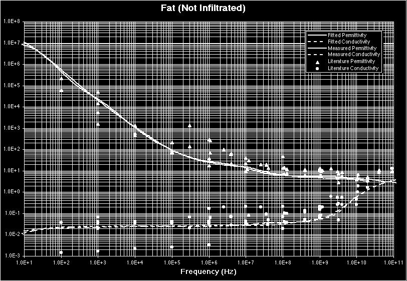
74 Figure A.1 Wet skin conductivity and permeability (measured vs. calculated) Figure A.2 Fat conductivity and permeability (measured vs. calculated)


 4 Dura")
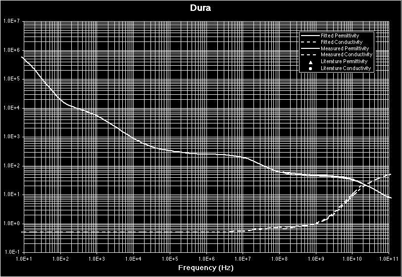
75 Figure A.3 Cortical bone conductivity and permeability (measured vs. calculated) Figure A.4 Dura conductivity and permeability (measured vs. calculated) 75
 Figure A.6 White matter conductivity and permeability (measured vs.")
76 Figure A.5 Grey matter conductivity and permeability (measured vs. calculated) Figure A.6 White matter conductivity and permeability (measured vs. calculated) 76

 8 Blood")
 77")
77 Figure A.7 CSF conductivity and permeability (measured vs. calculated) Figure A.8 Blood conductivity and permeability (measured vs. calculated) 77
Microsoft Word - EVS_ISO_IEC_27001;2014_et_esilehed.doc
 EESTI STANDARD EVS-ISO/IEC 27001:2014 INFOTEHNOLOOGIA Turbemeetodid Infoturbe halduse süsteemid Nõuded Information technology Security techniques Information security management systems Requirements (ISO/IEC
Microsoft PowerPoint - RRand_MEMS.ppt
 MEMS sensorid Rait Rand 1 Sissejuhatus MEMS MEMS : Micro-electromechanical systems 1974.a. rõhusensor masstoodangus 1988.a. mikromehhaanika ühendati elektroonikaga Süsteemina Sensorsüsteemid Aktuaatorsüsteemid
(Tõrked ja töökindlus \(2\))
)") Elektriseadmete tõrked ja töökindlus Click to edit Master title style 2016 sügis 2 Prof. Tõnu Lehtla VII-403, tel.6203 700 http://www.ttu.ee/energeetikateaduskond/elektrotehnika-instituut/ Kursuse sisu
Elektriseadmete tõrked ja töökindlus Click to edit Master title style 2016 sügis 2 Prof. Tõnu Lehtla VII-403, tel.6203 700 http://www.ttu.ee/energeetikateaduskond/elektrotehnika-instituut/ Kursuse sisu
Sissejuhatus GRADE metoodikasse
 Sissejuhatus GRADE metoodikasse Eriline tänu: Holger Schünemann ja GRADE working group www.gradeworkinggroup.org Kaja-Triin Laisaar TÜ peremeditsiini ja rahvatervishoiu instituut kaja-triin.laisaar@ut.ee
REQUEST FOR AN ASSIGNMENT OF LEI (fond) LEI KOODI MÄÄRAMISE TAOTLUS (fond) 1. FUND DATA / FONDI ANDMED: Legal Name / Ametlik nimi: Other Fund Names /
 LEI KOODI MÄÄRAMISE TAOTLUS (fond) 1. FUND DATA / FONDI ANDMED: Legal Name / Ametlik nimi: Other Fund Names /") REQUEST FOR AN ASSIGNMENT OF LEI (fond) LEI KOODI MÄÄRAMISE TAOTLUS (fond) 1. FUND DATA / FONDI ANDMED: Legal Name / Ametlik nimi: Other Fund Names / Fondi teised nimed: Business Register Number / Äriregistri
REQUEST FOR AN ASSIGNMENT OF LEI (fond) LEI KOODI MÄÄRAMISE TAOTLUS (fond) 1. FUND DATA / FONDI ANDMED: Legal Name / Ametlik nimi: Other Fund Names / Fondi teised nimed: Business Register Number / Äriregistri
PowerPoint Presentation
 Miks liituda projektiga LIFE Fit for REACH? Karin Viipsi Henkel Balti OÜ (Henkel Makroflex AS) Infopäev ettevõtetele, 09.11.2016 Sisukord Ettevõtte tutvustus Ettevõtte eesmärk projektis Mida on varasemalt
EESTI STANDARD EVS-EN :2000 This document is a preview generated by EVS Terastraat ja traattooted piirete valmistamiseks. Osa 4: Terastraadist
 EESTI STANDARD EVS-EN 10223-4:2000 Terastraat ja traattooted piirete valmistamiseks. Osa 4: Terastraadist keevitatud võrkpiire Steel wire and wire products for fences - Part 4: Steel wire welded mesh fencing
Võrguinverterite valik ja kasutusala päikeseelektrijaamades Robert Mägi insener
 Võrguinverterite valik ja kasutusala päikeseelektrijaamades Robert Mägi insener Robert Mägi o Õpingud: Riga Technical University o Haridus: MSc (Electrical Engineering) MSc (Automatic Telecommunications)
Language technology resources for Estonian text summarization Kaili Müürisep University of Tartu Institute of Computer Science
 Language technology resources for Estonian text summarization Kaili Müürisep University of Tartu Institute of Computer Science Outline Estonian language resources First experiment for summarization EstSum
EESTI STANDARD EVS-EN 1790:1999 This document is a preview generated by EVS Teemärgistusmaterjalid. Kasutusvalmid teekattemärgised Road marking materi
 EESTI STANDARD EVS-EN 1790:1999 Teemärgistusmaterjalid. Kasutusvalmid teekattemärgised Road marking materials - Preformed road markings EESTI STANDARDIKESKUS EESTI STANDARDI EESSÕNA NATIONAL FOREWORD Käesolev
Ppt [Read-Only]
![Ppt [Read-Only]](/thumbs/98/138481535.jpg "Ppt [Read-Only]") EL 2020 strateegia eesmärkidest, mis puudutab varajast koolist väljalangemist ja selle vähendamist EL 2020 strateegia eesmärkidest, mis puudutab madala haridustasemega noorte osakaalu vähendamist Madal
EL 2020 strateegia eesmärkidest, mis puudutab varajast koolist väljalangemist ja selle vähendamist EL 2020 strateegia eesmärkidest, mis puudutab madala haridustasemega noorte osakaalu vähendamist Madal
rp_ IS_3
 Page 1 of 5 Üldine informatsioon Kummelitee Exemption Flags Toote nimi Exempt from Artwork Exempt from NEP Reporting Country Lipton Brand Name CAMOMILE Product Name Legal Description Country Kummelitee
Inglise keele ainekava 5.klassile Kuu Õpitulemused Õppesisu Kohustuslik hindamine September 1. Räägib loomadest. Vaba aeg. Animals (Wild life 2. Kuula
 Inglise keele ainekava 5.klassile Kuu Õpitulemused Õppesisu Kohustuslik hindamine September 1. Räägib loomadest. Vaba aeg. Animals (Wild life 2. Kuulab, loeb ja jutustab dialooge and pets) Sõnavara teemadel
Slide 1
 TÖÖTUBA: ÕPIRÄNDE TUNNISTUSE TÄITMINE Margit Paakspuu 5163 Töötoa ülesehitus 1. Kellele ja milleks me õpirände tunnistusi väljastame? 2. Õpirände tunnistuse väljastamise protseduur 3. Õpirände tunnistuse
EESTI STANDARD EVS-ISO/IEC 25021:2014 This document is a preview generated by EVS SÜSTEEMI- JA TARKVARATEHNIKA Süsteemide ja tarkvara kvaliteedinõuded
 EESTI STANDARD SÜSTEEMI- JA TARKVARATEHNIKA Süsteemide ja tarkvara kvaliteedinõuded ja kvaliteedi hindamine (SQuaRE) Kvaliteedinäitajate elemendid Systems and software engineering Systems and software
Non-pharmacological treatment
 Tõendusmaterjali kokkuvõte - EvSu Kliiniline küsimus nr.4 Kas kõikidele dementsussündroomi kahtlusega patsientidele teha haiguse diferentsiaaldiagnostikaks strukturaalsed visualiseerimisuuringud (magnetresonantstomograafia
Microsoft PowerPoint - loeng2.pptx
 Kirjeldavad statistikud ja graafikud pidevatele tunnustele Krista Fischer Pidevad tunnused ja nende kirjeldamine Pidevaid (tihti ka diskreetseid) tunnuseid iseloomustatakse tavaliselt kirjeldavate statistikute
Kliiniliste soovituste koostamine
 Kliiniliste soovituste koostamine Eriline tänu: Holger Schünemann ja GRADE working group www.gradeworkinggroup.org Kaja-Triin Laisaar TÜ peremeditsiini ja rahvatervishoiu instituut kaja-triin.laisaar@ut.ee
Kuidas hoida tervist töökohal?
 Kuidas hoida tervist töökohal? Kristjan Port, TLU 25.04.2017 Tööinspektsiooni konverents Kas aeg tapab?. Mis on tervis? Teadmatus võib olla ratsionaalne. On olukordi milles teadmiste hankimise kulud ületavad
Tartu Ülikool
 Tartu Ülikool Code coverage Referaat Koostaja: Rando Mihkelsaar Tartu 2005 Sissejuhatus Inglise keelne väljend Code coverage tähendab eesti keeles otse tõlgituna koodi kaetust. Lahti seletatuna näitab
SQL
 SQL Kuues loeng 3GL inside 4GL Protseduurid Funktsioonid Tavalised Funktsioonid (üks väljund) Ilma väljundita Protseduurid Viitargumentide kasutamise võimalus Tabel-väljundiga Protseduurid Create function
Erasmus+: Euroopa Noored eraldatud toetused 2015 KA1 NOORTE JA NOORSOOTÖÖTAJATE ÕPIRÄNNE NOORTEVAHETUSED R1 1. taotlusvoor Taotleja Taotluse pealkiri
 Erasmus+: Euroopa Noored eraldatud toetused 2015 KA1 NOORTE JA NOORSOOTÖÖTAJATE ÕPIRÄNNE NOORTEVAHETUSED Loomade Nimel Baltic Animal Rights Gathering 2015 13270 Xploreworld Health in Action 20682 Ahtme
Microsoft Word - Loppukilpailu2015_16_tehtavat_viro_1
 Põhikooli matemaatika võistlus Lõppvõistlus reedel 22.1.2016 OSA 1 Lahendamiseks aega 30 min Punkte 20 Selles osas kalkulaatorit ei kasutata. Lühikesed lahendused ja vajalikud joonised teha samale paberile.
Kehtiv alates Vormi TSD lisa 3 Applicable from Annex 3 of Form 3 Unofficial translation Maksu- ja Tolliamet Estonian Tax and Cus
 Kehtiv alates 01.01.2018 Vormi TSD lisa 3 Applicable from 01.01.2018 Annex 3 of Form 3 Unofficial translation Maksu- ja Tolliamet Estonian Tax and Customs Board MITTERESIDENDIST JURIIDILISE ISIKU PÜSIVAST
SAF 7 demo paigaldus. 1.Eeldused SAF 7 demo vajab 32- või 64-bitist Windows 7, Window 8, Windows 10, Windows Server 2008 R2, Windows Server 2012, Wind
 SAF 7 demo paigaldus. 1.Eeldused SAF 7 demo vajab 32- või 64-bitist Windows 7, Window 8, Windows 10, Windows Server 2008 R2, Windows Server 2012, Windows Server 2012 R2, Windows Server 2016 või Windows
E-õppe ajalugu
 Koolituskeskkonnad MTAT.03.142 avaloeng Anne Villems September 2014.a. Põhiterminid Koolituskeskkonnad (Learning environments) IKT hariduses (ICT in education) E-õpe (e-learning) Kaugõpe (distance learning)
Ergonoomiliste riskide hindamine töökohal.
 Kas kontoritöötajad on tervemad kui tööstustöölised? Viive Pille Kutsehaiguste ja töötervishoiu keskus SA Põhja-Eesti Regionaalhaigla 26.05.2017 Euroopa töötajaskonna uuringust selgus, et 52% töötajaid
Avatud ja läbipaistev e-riik: Ees6 kui rajaleidja Andrus Kaarelson RIA peadirektori asetäitja riigi infosüsteemi alal 10. oktoober 2017
 Avatud ja läbipaistev e-riik: Ees6 kui rajaleidja Andrus Kaarelson RIA peadirektori asetäitja riigi infosüsteemi alal 10. oktoober 2017 Eesti kui rajaleidja e-riigi rajamisel E-teenused meie elu loomulik
Magnetic MRO
 3D-tehnoloogiad õhusõidukite hoolduses 3D Printimine / Virtuaalreaalsus/ 3D Skänneerimine Pärtel-Peeter Kruuv Interior Workshop supervisor Magnetic MRO Arendused: mis mõjutab, mida rakendada? IT Google
EESTI STANDARD EVS-ISO :2007 TRÜKITEHNOLOOGIA Protsessi kontrollimine pooltooni värvilahutuste, proovitrükkide ja tootmistrükkide valmistamisel
 EESTI STANDARD EVS-ISO 12647-1:2007 TRÜKITEHNOLOOGIA Protsessi kontrollimine pooltooni värvilahutuste, proovitrükkide ja tootmistrükkide valmistamisel Osa 1: Parameetrid ja mõõtmismeetodid (ISO 12647-1:2004)
Scanned Image
 EESTI MAAILMAS 21. SAJANDI KÜNNISEL EESTI MAAILMAS 21. SAJANDI KÜNNISEL TARTU ÜLIKOOL EESTI MAAILMAS 21. SAJANDI KÜNNISEL Eesti Vabariigi presidendi Lennart Meri 70. sünnipäevale pühendatud konverentsi
Slide 1
 Taimed ja sünteetiline bioloogia Hannes Kollist Plant Signal Research Group www.ut.ee/plants University of Tartu, Estonia 1. TAIMEDE roll globaalsete probleemide lahendamisel 2. Taimsete signaalide uurimisrühm
EESTI STANDARD EVS-ISO/IEC 27000:2015 This document is a preview generated by EVS INFOTEHNOLOOGIA Turbemeetodid Infoturbe halduse süsteemid Ülevaade j
 EESTI STANDARD INFOTEHNOLOOGIA Turbemeetodid Infoturbe halduse süsteemid Ülevaade ja sõnavara Information technology Security techniques Information security management systems Overview and vocabulary
Funktsionaalne Programmeerimine
 Kõrvalefektid ja Haskell Kõik senised programmid on olnud ilma kõrvalefektideta; so. puhtalt funktsionaalsed. Programmi täitmise ainsaks efektiks on tema väartus. Osade ülesannete jaoks on kõrvalefektid
Microsoft PowerPoint _04_20_Teadusest_ATI_tudengitele.pptx
 Tartu Ülikool Jaak Vilo 20. aprill 2009 Jaak Vilo 1 CV Karjääriredel Kuidas tehakse teadust Kuidas mõõta teadust Teadus on lahe saab teha mida tahad saab reisida lõpmatult saab suhelda lõpmatult PhD
Pöördumine Eesti Valitususe ja Europa Nõukogu Inimõiguste Komissari hr. Hammarbergi poole Appeal to the Government of the Republic of Estonia and the
 Pöördumine Eesti Valitususe ja Europa Nõukogu Inimõiguste Komissari hr. Hammarbergi poole Appeal to the Government of the Republic of Estonia and the Council of Europe Commissioner of Human Rights Mr.
EESTI STANDARD EVS-ISO/IEC/IEEE 15289:2013 This document is a preview generated by EVS SÜSTEEMI- JA TARKVARATEHNIKA Elutsükli infosaaduste (dokumentat
 EESTI STANDARD SÜSTEEMI- JA TARKVARATEHNIKA Elutsükli infosaaduste (dokumentatsiooni) sisu Systems and software engineering Content of life-cycle information products (documentation) (ISO/IEC/IEEE 15289:2011)
Microsoft Word - EVS_ISO_3574;2008_esilehed
 EESTI STANDARD EVS-ISO 3574:2010 KÜLMALT MÕÕTUVALTSITUD ÜLDTÖÖSTLUSLIKU KVALITEEDIGA JA TÕMBEKVALITEEDIGA SÜSINIKTERASLEHT Cold-reduced carbon steel sheet of commercial and drawing qualities EVS-ISO 3574:2010
Microsoft Word - C035736e.doc
 EESTI STANDARD Süsteemi- ja tarkvaratehnika Süsteemide ja tarkvara kvaliteedinõuded ja kvaliteedi hindamine (SQuaRE) Andmekvaliteedi mudel Software engineering Software product Quality Requirements and
ANOVA Ühefaktoriline dispersioonanalüüs Treeningu sagedus nädalas Kaal FAKTOR UURITAV TUNNUS Mitmemõõtmeline statistika Kairi Osula 2017/kevad
 ANOVA Ühefaktoriline dispersioonanalüüs Treeningu sagedus nädalas Kaal FAKTOR UURITAV TUNNUS Factorial ANOVA Mitmefaktoriline dispersioonanalüüs FAKTOR FAKTOR Treeningu sagedus nädalas Kalorite kogus Kaal
EESTI STANDARD EVS-ISO/IEC :2005 This document is a preview generated by EVS INFOTEHNOLOOGIA Avatud süsteemide vastastikune ühendamine Tehingut
 EESTI STANDARD EVS-ISO/IEC 10026-1:2005 INFOTEHNOLOOGIA Avatud süsteemide vastastikune ühendamine Tehingute hajustöötlus Osa 1: OSI TP mudel Information technology Open Systems Interconnection Distributed
tallinn arvudes 2003.indd
 15 16 Ilmastik ja keskkond 1. Õhutemperatuur, 2003... 18 2. Päikesepaiste, 2003.... 19 3. Sademed, 2003... 20 4. Keskmine tuule kiirus, 2003.. 21 5. Looduskaitse load, 2003..... 22 6. Õhusaaste paiksetest
Väljaandja: Vabariigi Valitsus Akti liik: välisleping Teksti liik: algtekst Jõustumise kp: Avaldamismärge: RT II 2010, 18, 90 Eesti Vabarii
 Väljaandja: Vabariigi Valitsus Akti liik: välisleping Teksti liik: algtekst Jõustumise kp: 04.06.2010 Avaldamismärge: RT II 2010, 18, 90 Eesti Vabariigi ja Soome Vabariigi viisaküsimustes esindamise kokkulepete
Microsoft Word - 08.doc
 EESTI VÕIMALIK RAHVAARV JA VANUSKOOSSEIS AASTANI 2050 Aasa Maamägi Rahvastikustatistika talituse juhtivstatistik 2000. aasta rahva- ja eluruumide loenduse alusel Statistikaametis koostatud vaadeldava ajaperioodi
SQL
 SQL Teine loeng Mõtelda CREATE TABLE ( { INTEGER VARCHAR(10)} [ NOT NULL] ); Standard SQL-86 (ANSI X3.135-1986), ISO võttis üle 1987 SQL-89 (ANSIX3.135-1989) SQL-92 (ISO/IEC 9075:1992)
Baltic Retail Forum 2019 Baltic Retail Forum on konverents jaekaubanduse juhtidele. Arutleme uueneva tehnoloogia arengusuundade üle, analüüsime
 Baltic Retail Forum 2019 Baltic Retail Forum 2019 - on konverents jaekaubanduse juhtidele. Arutleme uueneva tehnoloogia arengusuundade üle, analüüsime kaubandussektori väljavaateid, otsime õigeid vastuseid
EESTI KUNSTIAKADEEMIA
 HIGHER EDUCATION INSTITUTIONS in Estonia (1990-2011) Estonian ENIC/NARIC 2012 1 The current document comprises a list of public universities, state professional higher education institutions, private higher
Microsoft PowerPoint - TÜ TVT - Kavandamine ja arhitektuur 2.ppt
 Kavandamine ja arhitektuur Erik Jõgi erik.jogi@hansa.ee Muutused Muutused on elu igapäevane osa Meie peame tagama, et meie kirjutatud tarkvara need muutused üle elab Oleme valmis muutusteks, mitte ei võitle
(loeng3-ohtlikud_koodiloigud)
") #include int main (void) uint8_t arr[] = 0x11, 0x22 uint16_t *ptr; ptr = (uint16_t*)&arr[0]; printf ("arr: 0x%02x, 0x%02x\n", arr[0], arr[1]); printf ("ptr: 0x%04x\n", *ptr); /* vigane pointeri
#include int main (void) uint8_t arr[] = 0x11, 0x22 uint16_t *ptr; ptr = (uint16_t*)&arr[0]; printf ("arr: 0x%02x, 0x%02x\n", arr[0], arr[1]); printf ("ptr: 0x%04x\n", *ptr); /* vigane pointeri
III OSA. RAADIOSAGEDUSALA 3600 MHz 1000 GHz Rahvusvahelise Telekommunikatsiooni Liidu konventsiooni ja põhikirja täiendavate raadioeeskirjadega määrat
 III OSA. RAADIOSAGEDUSALA 3600 MHz 1000 GHz Rahvusvahelise Telekommunikatsiooni Liidu konventsiooni ja põhikirja täiendavate raadioeeskirjadega määratud raadiosagedusala kasutusrežiim ja otstarve 3600
PowerPoint Presentation
 Ülevaade Mehhaanika ja elektroonika tooted, elektromehaanilised koosted 30 aastat kogemust Müügikäive 2018 MEUR 15,4 2 tootmisüksust Euroopas HYRLES OY Soome tehas Asutatud 1989 Tootmine 8500 m2 Personal
Powakaddy
 Powakaddy PowaKaddy Sport http://www.powakaddy.com/index.php/electric-trolleys/sport.html Elektrilised kärud liitium või tavalise akuga / Electrical trolleys with lithium or acid battery Liitium akuga
Rahvusvaheline motokross Baltimere Karikas 2015 Soome Eesti Läti Leedu Kooskõlastanud: EMF-i alajuht; Kinnitanud: EMF peasekretär 1. Aeg ja koht: 18.0
 Rahvusvaheline motokross Baltimere Karikas 2015 Soome Eesti Läti Leedu Kooskõlastanud: EMF-i alajuht; Kinnitanud: EMF peasekretär 1. Aeg ja koht: 18.04.2015, Eesti, Holstre-Nõmme motokeskus. (58 o 18 56.36
Microsoft Word - EVS_ISO_31000;2010_et_esilehed
 EESTI STANDARD EVS-ISO RISKIJUHTIMINE Põhimõtted ja juhised Risk management Principles and guidelines EVS-ISO EESTI STANDARDI EESSÕNA NATIONAL FOREWORD Käesolev Eesti standard EVS-ISO Riskijuhtimine. Põhimõtted
Microsoft PowerPoint IntroRiskAnal.ppt
 SISSEJUHATUS RISKIANALÜÜSI VETERINAARSES RAHVATERVISHOIUS Arvo Viltrop EMÜ VLI 1 Kasutatud allikad Woolridge ja Kelly Risk Analysis Course (2000) Vose Consulting Quantitative Risk Assessment for Animal
Microsoft Word - EVS_ISO_6743_13;2012_et_en
 EESTI STANDARD Avaldatud eesti keeles: juuli 2012 Jõustunud Eesti standardina: juuli 2012 MÄÄRDEAINED, TÖÖSTUSÕLID JA NENDEGA SEOTUD TOOTED (KLASS L) Klassifikatsioon Osa 13: tüüp G (juhikud) Lubricants,
Microsoft Word - MM_17 13[1] lisa 3
![Microsoft Word - MM_17 13[1] lisa 3](/thumbs/98/138438163.jpg "Microsoft Word - MM_17 13[1] lisa 3") Lisa 3 majandus- ja kommunikatsiooniministri 2006.a määrusele nr CEPT ELEKTROONILISE SIDE KOMITEE OTSUSED JA SOOVITUSED, ITU SOOVITUSED, EUROOPA LIIDU DIREKTIIVID JA OTSUSED, RAHVUSVAHELISED KOKKULEPPED,
Lisa 3 majandus- ja kommunikatsiooniministri 2006.a määrusele nr CEPT ELEKTROONILISE SIDE KOMITEE OTSUSED JA SOOVITUSED, ITU SOOVITUSED, EUROOPA LIIDU DIREKTIIVID JA OTSUSED, RAHVUSVAHELISED KOKKULEPPED,
Microsoft Word - EVS_EN_61557_5;2007_et.doc
 EESTI STANDARD Avaldatud eesti keeles: jaanuar 2009 Jõustunud Eesti standardina: mai 2007 ELEKTRIOHUTUS MADALPINGEVÕRKUDES VAHELDUVPINGEGA KUNI 1000 V JA ALALISPINGEGA KUNI 1500 V Kaitsesüsteemide katsetus-,
Vorm_V1_2014_18.02
 Kehtiv alates jaanuar 2014 Applicable from 2014 Maksu- ja Tolliamet Tax and Customs Board Vorm V1 Form V1 MITTERESIDENDI JA LEPINGULISE INVESTEERIMISFONDI EESTIS ASUVA VARA VÕÕRANDAMISEST SAADUD KASU DEKLARATSIOON
 Riistvara kirjelduskeel VHDL L4, L5. Riistvara kirjelduskeel VHDL L6. Mäluga süsteemid VHDL-s L7. VHDL ja süntees 1 Atribuudid Atribuut on väärtus, funktsioon, tüüp, vahemik, signaal või konstant, mida
  Andmebaasid (6EAP) I praktikum Mida praktikumides tehakse? Õpitakse SQL i Tehakse andmebaas ope (igas praktikumis natuke, kuni lõpuks saab valmis) Tehakse andmebaas edu (kui ope on valmis, tehakse edu,